How to swing a SkyKatana in Subaru HSC-SSP
This example provides a guide for using SkyKatana to construct a mask for a small region of the HSC-SSP survey. It will help you to familiarize with key concepts, methods and serve as a model workflow for processing larger, more sophisticated masks.
The main class is called SkyMaskPipe. After a pipeline is instantiated, you can add masks (a.k.a. maps) due to various effects. These masks are independent boolean (or bit-packed boolean) healsparse maps we call stages. Stages are stored within the class along with some metadata and some typical stages are:
- footmask :: holds the footprint map created by pixelating discrete sources of a catalog
- patchmask :: holds the map created from HSC patches matching some criteria
- propmask :: mask created from the combination of multiple healsparse propery maps matching some criteria
- circmask :: mask created from a list of circular sources, usually stars
- boxmask :: map created from a set of box regions
- ellipmask :: map created from a set of elliptical regions
Once you have a few stages in the pipeline, their masks can be combined by combine() into:
- mask :: mask generated from the logical combination of the maps above
Example dataset
We have prepared a small dataset of ~8 million HSC galaxies. It contains a HATS catalog and auxiliary input files used below. Download (170 MB), decompress it, and then adjust the folder location in BASEPATH.
Imports and input data files
We should start by importing SkyMaskPipe, which is the main Skykatana class, along with some auxiliary packages.
from skykatana import SkyMaskPipe
import matplotlib.pyplot as plt
from pathlib import Path
import astropy.units as u
from astropy.coordinates import SkyCoord
import lsdb          # if pixelating source catalogs in HATS format
Throughout this example, SkyKatana will read and pixelate discrete sources and many geometrical shapes. Concentrate their location paths here.
# Base path of the example dataset
BASEPATH = Path('../../skykatana_example_data/example_data/')
# Input HATS catalog (these are HSC galaxies)
HATSCAT = BASEPATH / 'hscx_minispring_gal/'
# Bright stars in HSC area
STARS_REGIONS     = BASEPATH / 'hsc_aux/stars_iband.parquet'
# Boxes around stars in HSC
BOX_STARS_REGIONS = BASEPATH / 'hsc_aux/starboxes_iband.parquet'
# HSC patches and QA patch list. See here for details -> hsc-release.mtk.nao.ac.jp/schema/#pdr3.pdr3_wide.patch_qa
PATCH_FILE     = [BASEPATH / 'hsc_aux/tracts_patches_minispring.parquet']
QA_FILE        = BASEPATH / 'hsc_aux/patch_qa.csv'
# SFD dust extintion map (precut to the region covered in this example)
PROPMAP_FILE   = BASEPATH / 'hsc_aux/sfd_ebv_piece.fits'
# Some dummy geometrical regions
ELLIP_REGIONS       = BASEPATH / 'hsc_aux/extended_sources.dat'
USER_CIRCLE_REGIONS = BASEPATH / 'hsc_aux/user_circs.dat'
USER_POLY_REGIONS   = BASEPATH / 'hsc_aux/user_polys.dat'
USER_ZONE_REGIONS   = BASEPATH / 'hsc_aux/user_zones.dat'
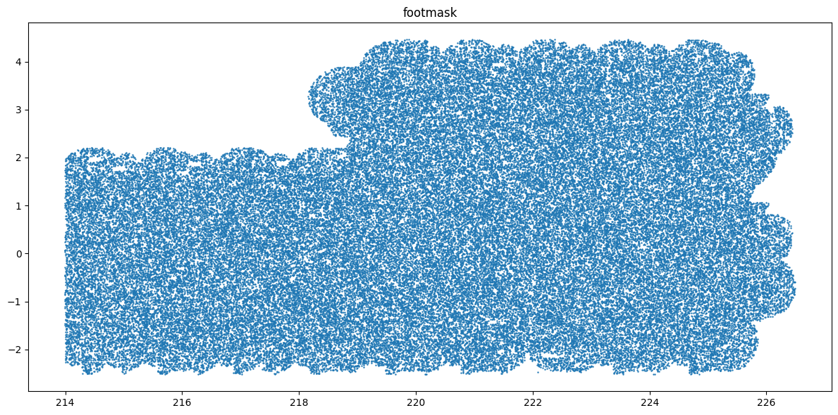
1. Instantiate and add a footprint stage
We choose an ouput sparse order now (though we can change it later) and create an empty SkyMaskPipe object mkp. We will first add a footprint stage, i.e. a stage defined by the pixelization of the discrete sources in our HATS catalog.
mkp = SkyMaskPipe(order_out=15)
mkp.build_foot_mask(sources=lsdb.open_catalog(HATSCAT), order_foot=13);
    BUILDING FOOT MASK >>>>>>>>>>>>>>>>>>>>>>>>>>>>>>>>>>>>>>>>>>>>>>
        Order :: 13
    --- Pixelating HATS catalog
    --- Foot mask area                         : 69.35790724770318
Note we selected a smaller order, as it is more compatible to produce a continuous coverage given the the density of sample. Every stage can be pixelized at different order and is only during combination that the ouput mask will be produced at order_out. The result is a footmask stage accesible as mkp.footmask.
2. Add a second stage from HSC-SSP patches
The HSC-SSP survey is divided into "patches" which are the fundamental areal units that result from diving each tract into smaller ~12 arcmin side equi-area rectangular regions. A number of QA measurements are available per patch indicating for example the limiting psf magnitude in a given band. Create now a patchmask stage after filtering out patches below a given depth threshold in gri bands.
filt = "(gmag_psf_depth>26.2) and (rmag_psf_depth>25.9) and (imag_psf_depth>25.7)"
mkp.build_patch_mask(patchfile=PATCH_FILE, qafile=QA_FILE, filt=filt, order_patch=13);
    BUILDING PATCH MAP >>>>>>>>>>>>>>>>>>>>>>>>>>>>>>>>>>>>>>>>>>>
    --- Processing ../../skykatana_example_data/example_data/hsc_aux/tracts_patches_minispring.parquet
        Order :: 13
        Patches with QA                       : 3708
        Patches with QA fulfilling conditions : 2003
        Surviving patch pixels                : 1062650
    --- Patch mask area                           : 54.43575391135537
Inspecting pipelines
Just typing mkp disaplays the list of stages stored in the pipeline, along with useful information such as coverage order/nside, sparse order/nside, number of valid pixels (e.g. True pixels) and the pixel size at the sparse order. This is ultimately the resolution of the stage map.
    footmask       : (ord/nside)cov=4/16   (ord/nside)sparse=13/8192  valid_pix=1353948  area= 69.36 deg² pix_size=  25.8"
    patchmask      : (ord/nside)cov=4/16   (ord/nside)sparse=13/8192  valid_pix=1062650  area= 54.44 deg² pix_size=  25.8"
3. Add stages for bright stars
The effect of bright stars in HSC can be decomposed into circular shapes due to the bright halo of stars, and into rectangular boxes due to saturated bleed trails along the CCD. SkyKatana has methods to pixelize both, creating a circmask and a boxmask stage.
mkp.build_circ_mask(data=STARS_REGIONS, fmt='parquet');
mkp.build_box_mask(data=BOX_STARS_REGIONS, fmt='parquet');
    BUILDING CIRCLES MASK >>>>>>>>>>>>>>>>>>>>>>>>>>>>>>>>>>>>>
    --- Pixelating circles from ../../skykatana_example_data/example_data/hsc_aux/stars_iband.parquet
        Order :: 15 | pixelization_threads=4
        Circles to pixelate: 223015 in batches of 600000
            processing circles 0:223015 ...
    --- Circles mask area                        : 12.277230882152068
    BUILDING BOXES MASK >>>>>>>>>>>>>>>>>>>>>>>>>>>>>>>>>>>>>>>>
    --- Pixelating boxes from ../../skykatana_example_data/example_data/hsc_aux/starboxes_iband.parquet
        Order :: 15
        done
    --- Boxes mask area                           : 5.564107952862163
4. Mask out extended sources
Large nearby galaxies and other extended objects will usually get deblended into multiple sources that get into large survey databases. Sometimes it is not straightforward to assign a single parent object so that, depending on your purposes, it could be more practical to just mask out an elliptical region around them. For didactic purposes, we will pixelize three huge dummy galaxies.
    BUILDING ELLIPSES MASK >>>>>>>>>>>>>>>>>>>>>>>>>>>>>>>>>>>>>
    --- Pixelating ellipses from ../../skykatana_example_data/example_data/hsc_aux/extended_sources.dat
        Order :: 15
        done
    --- Ellipses mask area                        : 0.5414152216851591
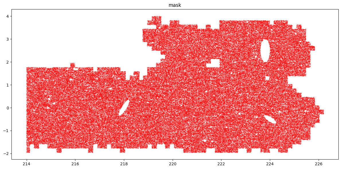
5. Combine stages
Now combine into a "final" mask by intersecting footmask with patchmask, subtracting circmask/boxmask (e.g. due to stars), and ellipmask (e.g. due to large galaxies). If maps have different geometry such as sparse or coverage order, they will be reprojected on the fly to allow combination. SkyKatana streaming algorithms allow fast reprojections of masks composed of billions of pixels in "harsh" low-memory environments of
even 16GB RAM. We specify a list of positive areas (that we want to keep) and a list of negative areas (that we want to subtract).
mkp.combine(positive=[('footmask','patchmask')], negative=['circmask','boxmask','ellipmask'], verbose=True);
    [combine] aligning coverage for 'footmask' : c4 → c4
    [combine] aligning coverage for 'patchmask' : c4 → c4
    [combine] aligning coverage for 'circmask' : c4 → c4
    [combine] aligning coverage for 'boxmask' : c4 → c4
    [combine] aligning coverage for 'ellipmask' : c4 → c4
    [combine] target=(o15, c4), work_order=13, r2=16
    [combine:&] group of 2 stages: orders=[13, 13] -> work 13
    [combine] done: order_out=15 (NSIDE=32768), order_cov=4 (NSIDE=16), valid_pix=14,312,202, area=45.823 deg², bit_packed=True
Inspect the pipeline and note now there is a new mask stage.
    footmask       : (ord/nside)cov=4/16   (ord/nside)sparse=13/8192  valid_pix=1353948  area= 69.36 deg² pix_size=  25.8"
    patchmask      : (ord/nside)cov=4/16   (ord/nside)sparse=13/8192  valid_pix=1062650  area= 54.44 deg² pix_size=  25.8"
    circmask       : (ord/nside)cov=4/16   (ord/nside)sparse=15/32768 valid_pix=3834656  area= 12.28 deg² pix_size=   6.4"
    boxmask        : (ord/nside)cov=4/16   (ord/nside)sparse=15/32768 valid_pix=1737887  area=  5.56 deg² pix_size=   6.4"
    ellipmask      : (ord/nside)cov=4/16   (ord/nside)sparse=15/32768 valid_pix=169105   area=  0.54 deg² pix_size=   6.4"
    mask           : (ord/nside)cov=4/16   (ord/nside)sparse=15/32768 valid_pix=14312202  area= 45.82 deg² pix_size=   6.4"
combine() can perform the union --specified between braquets []-- and the intersection --specified between parenthesis()-- of any stage specified in the positive group. For example, the following would intersect footmask with patchmask, join the result with zonemask and subtract the three masks for circles, boxes and ellipses.
some_map = mkp.combine(positive=[('footmask','patchmask'),'zonemask'], negative=['circmask','boxmask','ellipmask'])
Overwriting stages
All build_* methods modify (and overwrite) its corresponding stage unless output_stage is specified.
Independent of that, all build_* methods also return the new stage so it can get assigned to any variable outside
of the pipeline.
6. Generate randoms & apply mask to catalog
Before visualizing our pipeline, lets dive first into some applications. One of the most useful applications is generating random points uniformly distributed over the healpix pixels of a stage, e.g. to construct syntetic catalogs for computing two-point correlation functions. SkyKatana implements fast alogrithms that work without materializing the global valid-pixels list, enabling such computations with billion pixel masks.
Lets generate 1 million randoms over the mask stage:
| ra | dec |
|---|---|
| float64 | float64 |
| 217.0317095518112 | 0.7331634065253888 |
| 224.5373511314392 | 3.0642220551410375 |
| 217.44206607341766 | 1.7395248080214378 |
| 221.71443343162534 | 1.0998600539612031 |
| 216.9879573583603 | -1.1881555807593203 |
Of course you can use any stage stage, and also save the table in parquet format when file is specified, e.g. file='ellip_randoms.parquet'
rands_in_holes = mkp.makerans(stage='ellipmask', nr=100_000, file='ellip_randoms.parquet')
rands_in_holes[:5]
| ra | dec |
|---|---|
| float64 | float64 |
| 223.81314396858212 | 2.687722491092348 |
| 223.7549990415573 | 2.795585374635337 |
| 223.75130295753476 | 2.6220092843271305 |
| 223.80658864974973 | 2.18948552704603 |
| 223.62743854522705 | 2.3103729155855297 |
Another very relevant use of masks is returning the sources of a given catalog that fall inside. The apply() method is designed to do that.
import lsdb
cat = lsdb.read_hats(HATSCAT, columns=['ra','dec']).compute()
srcs_masked = mkp.apply(stage='mask', cat=cat, columns=['ra','dec'])
7. Saving/reading pipelines
Use write() to save a complete SkyMaskPipe object to disk. This will create a directory where each stage is saved in FITS format using bit-encoding compression, plus a JSON file holding various metadata. Once again, just plain dumping pixels to a hard drive would be very inefficient, so SkyKatana implements special compression algorithms that balance speed, memory usage and file size. For referece, a 0.5 billion pixel mask should be writen to disk in a few seconds, read back in under a minute, and occupy ~300 MB.
When you need to read back a pipeline, use the read() method:
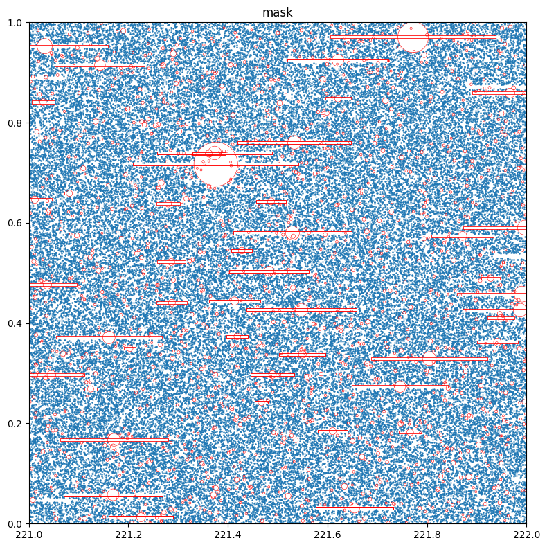
8. Plotting and visualizing masks
The plot() method is suitable for very fast visualizations by plotting random (ra,dec) sources over a given stage
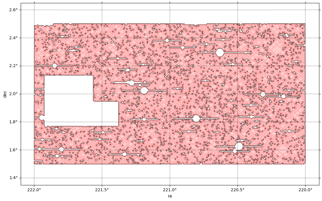
Plot a zoom of mask, overlaying the circles and boxes associated to the stars masked out by passing plot_circles and plot_boxes. The clipra and clipdec parameters allow to specify a plotting window.
# Define two dictionaries with data files, format and column names
stars={'data':str(STARS_REGIONS), 'fmt':'parquet', 'columns':['ra','dec','radius']}
boxes={'data':str(BOX_STARS_REGIONS), 'fmt':'parquet', 'columns':['ra_c','dec_c','width','height']}
mkp.plot(stage='mask', nr=4_000_000, figsize=[8,8], clipra=[221,222], clipdec=[0,1], plot_circles=stars, plot_boxes=boxes)
While plotting randoms can be fast, if the mask is large we need to generate lots of randoms to reach an adequate density. Moreover, points are drawn respect to simple x-y cartesian axes. An alternative is to represent masks with their MOCs. A MOC (Multi-Order Coverage map) is a data structure that defines the coverage of complex sky regions by a series of disjoint healpix pixels of multiple resolutions. Using the great capabilities of mocpy, the method plot_moc() generates accurrate visualizations in WCS (World Coordinate System) axes with a variety of astronomical projections.
center = SkyCoord(220*u.deg, 1*u.deg)   # specify the center of plot
fov    = 8 * u.deg                      # specify the field of view
fig, ax, wcs = mkp.plot_moc(stage='footmask', center=center, fov=fov, color='b') # MOC of footmask
fig, ax, wcs = mkp.plot_moc(stage='patchmask', ax=ax, wcs=wcs, color='g')        # MOC of patchmask
    Looking pixels...
    Found 1353948 pixels
    Creating display moc from pixels...
    MOC max_order is 13 --> degrading to 11...
    Drawing plot...
    Looking pixels...
    Found 1062650 pixels
    Creating display moc from pixels...
    MOC max_order is 13 --> degrading to 11...
    Drawing plot...
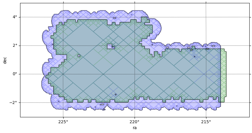
It can be readly seen above that keeping only the patches above a minimum deph has indeed discared the border areas of the survey, which are covered by less visits than the central areas and therefore do not reach the same depth after coaddition.
Now make zoom on a MOC. When zooming by selecting a smaller FOV, millions of high order pixels can show up and slow down plotting and/or consume large ammounts of memory. Use clipra/clipdec to specify a region of interest and avoid processing pixels outside the chosen display window.
center = SkyCoord(221*u.deg, 2*u.deg)    # center of plot
fov    = [2.2*u.deg, 1.3*u.deg]          # field of view
clipra = [220, 222]                      # ra limits for processing pixels
clipdec = [1.5, 2.5]                     # dec limits for processing pixels
fig, ax, wcs = mkp.plot_moc(stage='mask',  center=center, fov=fov,  color='r', clipra=clipra, clipdec=clipdec, figsize=[13,8])
    Looking pixels inside clip box...
    Found 504524 pixels
    Creating display moc from pixels...
    MOC max_order is 15 --> no degrading...
    Drawing plot...
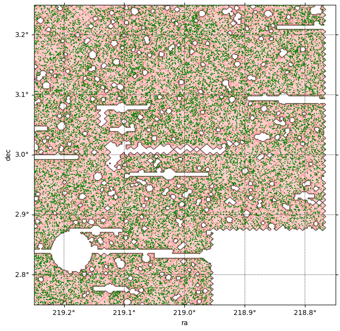
At some point it might be desirable to plot actual sources to check where they fall respecto to a mask. Lets plot the MOC and overlay a catalog sources with plot_srcs(). In this case we shall plot the sources we already applied mask before. If math was correct, not a single source should lie outside the MOC.
center = SkyCoord(219*u.deg, 3*u.deg)    # center of plot
fov    = [0.5*u.deg, 0.5*u.deg]          # field of view
clipra = [218.5, 219.3]                  # ra limits for processing pixels
clipdec = [2.7, 3.5]                     # dec limits for processing pixels
fig, ax, wcs = mkp.plot_moc(stage='mask',  center=center, fov=fov,  color='r', alpha=0.2, clipra=clipra, clipdec=clipdec, figsize=[8,8])
fig, ax, wcs = mkp.plot_srcs(srcs_masked['ra'], srcs_masked['dec'], ax=ax, wcs=wcs, s=10, alpha=1, color='g', zorder=10)
    Looking pixels inside clip box...
    Found 99104 pixels
    Creating display moc from pixels...
    MOC max_order is 15 --> no degrading...
    Drawing plot...
9. Build methods: from geometry to masks
Skykatana has methods to pixelate and generate masks from a variety of geometric shapes.
mkp.build_foot_mask(sources=lsdb.open_catalog(HATSCAT));                      # from individual point sources
mkp.build_prop_mask(prop_maps=PROPMAP_FILE,thresholds=1.3,comparisons='lt');  # from healsparse property maps
mkp.build_circ_mask(data=STARS_REGIONS, fmt='parquet');                       # from circular regions
mkp.build_box_mask(data=BOX_STARS_REGIONS, fmt='parquet');                    # from box regions
mkp.build_ellip_mask(data=ELLIP_REGIONS, fmt='ascii');                        # from elliptical regions
mkp.build_poly_mask(data=USER_POLY_REGIONS, fmt='ascii');                     # from quadrangular sky polygons
mkp.build_zone_mask(data=USER_ZONE_REGIONS, fmt='ascii');                     # from zones delimited by ra-dec boundaries
mkp.build_patch_mask(patchfile=PATCH_FILE, qafile=QA_FILE, filt=filt);        # from a sets of patches with custom filtering
Each the these build_* methods store its calling arguments as dictionaries under _params. In this way, all the metadata used to create each stage is saved in the pipeline and kept for record. Use stage_meta() to quickly access the metadada associated with a stage.
    {'sources': '../../skykatana_example_data/example_data/hscx_minispring_gal',
     'order_foot': 13,
     'order_cov': 4,
     'columns': ('ra', 'dec'),
     'remove_isopixels': False,
     'erode_borders': False,
     'bit_packing': True,
     'pixels': np.int64(1353948),
     'area_deg2': np.float64(69.35790724770318)}
mkp._params['footmask']. Access all dictionaries with mkp._params.
10. Creating masks from property maps
While patches are geometric constructions specific to HSC, in general you can might also need to restrict to arbitrary areas meeting certain conditions. Surveys like Rubin produce healsparse propery maps, which track spatial information about the survey (e.g. observing conditions, depth, exposure time) in a dual healpix map constructed at coarse and sparse orders.
The map file below contains a small region of the dust extinction map of Schlegel, Finkbeiner & Davies in healsparse format. We impose and arbitrary cut to discard areas with very high extinction and intersect footmask, patchmask and propmask
mkp.build_prop_mask(prop_maps=PROPMAP_FILE,thresholds=1.3,comparisons='lt')
mkp.combine(positive=[('footmask','patchmask','propmask')]);
    BUILDING PROPERTY MAP >>>>>>>>>>>>>>>>>>>>>>>>>>>>>>>>>>>>>
    --- Processing ../../skykatana_example_data/example_data/hsc_aux/sfd_ebv_piece.fits
    --- Propertymap coverage order changed to 4
    --- Propertymap sparse order changed to 15
    --- Propertymap mask area                       : 113.86116591708016
    [combine] aligning coverage for 'footmask' : c4 → c4
    [combine] aligning coverage for 'patchmask' : c4 → c4
    [combine] aligning coverage for 'propmask' : c4 → c4
    [combine] target=(o15, c4), work_order=13, r2=16
    [combine:&] group of 3 stages: orders=[13, 13, 15] -> work 13
    [combine] done: order_out=15 (NSIDE=32768), order_cov=4 (NSIDE=16), valid_pix=14,497,392, area=46.416 deg², bit_packed=True
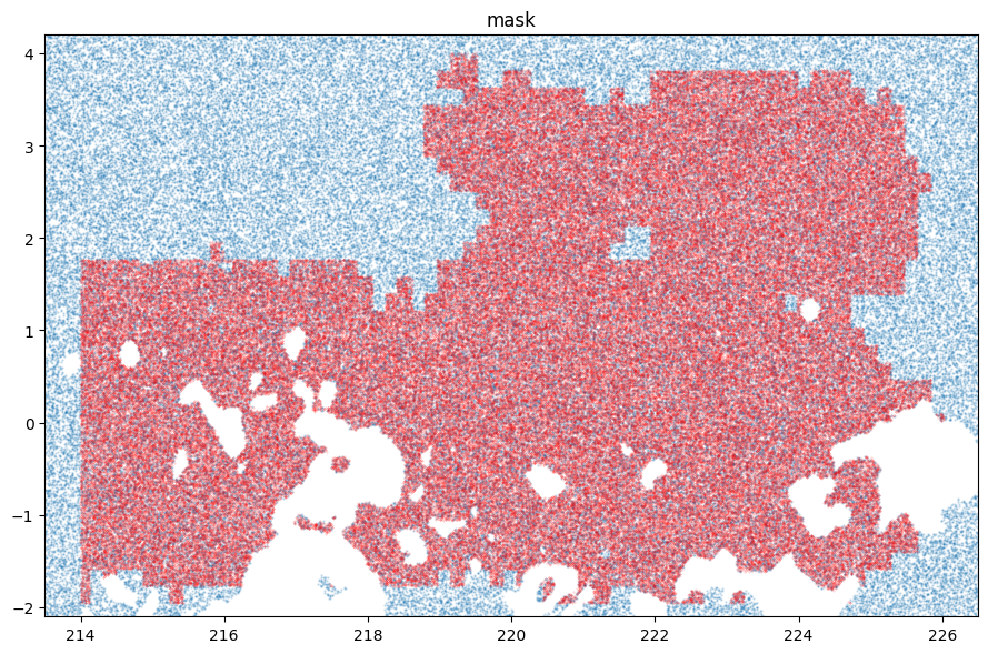
Overlay the SFD extincion map in propmask and the new combined final mask
fig, ax = plt.subplots(figsize=[9,6])
mkp.plot(stage='propmask', nr=200_000, alpha=0.2, clipra=[213.5, 226.5], clipdec=[-2.1,4.2], ax=ax)
mkp.plot(stage='mask', nr=200_000, s=0.09, color='r', alpha=0.3 , ax=ax)
11. Creating stages with custom names
All build_* methods create a stage with a fixed name, e.g. footmask, propmask, circmask, etc. These area canonical names chosen to help structuring your pipleline, but SkyKatana
is not rectricted in that aspect. You can add your own stages with any name (or origin) as long as they are valid healsparse
boolean (or bit-packed boolean) masks. The build_* methods support an output_stage keyword to specify stages with custom names, and they will also store on each call the corresponding dictionary with calling parameters under _params.
Lets use build_circ_mask() to create bogus masks due to two different star catalogs and store them with custom names (do not excute the cells below unless you supply the input files).
mkp.build_circ_mask(data='statcat1.parquet', fmt='parquet', output_stage = 'stars1_mask');
mkp.build_circ_mask(data='statcat2.parquet', fmt='parquet', output_stage = 'stars2_mask');
    stars1_mask       : (ord/nside)cov=4/16   (ord/nside)sparse=15/32768 valid_pix=3834656  area= 12.28 deg² pix_size=   6.4"
    stars2_mask       : (ord/nside)cov=4/16   (ord/nside)sparse=15/32768 valid_pix=1730710  area= 6.02 deg² pix_size=   6.4"
Lets create a bogus cirrus mask using plain mocpy, and add it to a pipeline:
import healsparse as hsp, numpy as np
from mocpy import MOC
from astropy.coordinates import SkyCoord
moc = MOC.from_zone(SkyCoord([[220, -5], [222, 0.3]], unit="deg"), max_depth=15)
cirrus = hsp.HealSparseMap.make_empty(2**4, 2**15, dtype=np.bool_)
pixels = moc.flatten().astype(np.int64)
cirrus.update_values_pix(pixels, True)
cirrusmask = cirrus.as_bit_packed_map()

mkp.cirrusmask = cirrusmask
Then, you can work, combine and plot as with any other stage as normal.
mkp.combine(positive=['footmask','patchmask','cirrusmask'], negative=['stars1_mask','stars2_mask','ellipmask']);
Naming stages
Note that while any name is valid for a stage, only stages ending with "mask" show up when printing, e.g cirrusmask,
satellitemask, nebulamask, etc., and most build_* methods will only accept output_stage names ending
with "mask".